Multi-Cylinder Series — Summary and Master Comparison

Series: ← The Slider-Crank, Three Ways · ← Multi-Cylinder I4 · ← Boxer-4 · ← Rocking Couples · ← Non-boxer Flat-4 · Summary · V-Engines → · Combustion → · Balance Shafts → · Engine Mounts → · Active Damping → · Chassis Response → · Engine Mounts →

Reference: Field Guide · Concepts Primer · Physics · Computational Machinery · Dimensional Reduction

A capstone chapter collecting the results from the entire multi-cylinder series into one table, one comparison plot, one parametric sweep, and an FAQ that closes the loop with the textbook rod-ratio theory.

The script that does all of it: engine_comparison.py. Pick an RPM and an R/L ratio, and it runs the single-cylinder simulation once and phasor-sums it into every layout we’ve covered.

1. The six in-scope configurations

Each one is defined entirely by three lists (per-cylinder kinematic phases, ±1 signs for mirror-opposed banks, positions along the crankshaft). That’s everything the phasor framework needs.

Layout	Phases (deg)	Signs	Positions (in units of `a`)
Single cylinder	`[0]`	`[+1]`	`[0]`
Straight-3	`[0, 120, 240]`	`[+1, +1, +1]`	`[−a, 0, +a]`
Inline-4 (I4)	`[0, 180, 180, 0]`	`[+1, +1, +1, +1]`	`[−3a, −a, +a, +3a]`
Boxer-4	`[0, 0, 180, 180]`	`[+1, −1, +1, −1]`	`[−a, −a, +a, +a]`
Non-boxer flat-4	`[0, 180, 180, 0]`	`[+1, −1, +1, −1]`	`[−a, −a, +a, +a]`
Straight-6 (I6)	`[0, 120, 240, 240, 120, 0]`	`[+1,+1,+1,+1,+1,+1]`	`[−5a/2, −3a/2, −a/2, +a/2, +3a/2, +5a/2]`

These populate every cell of the (Force, Moment) outcome table we’ll see in §3.

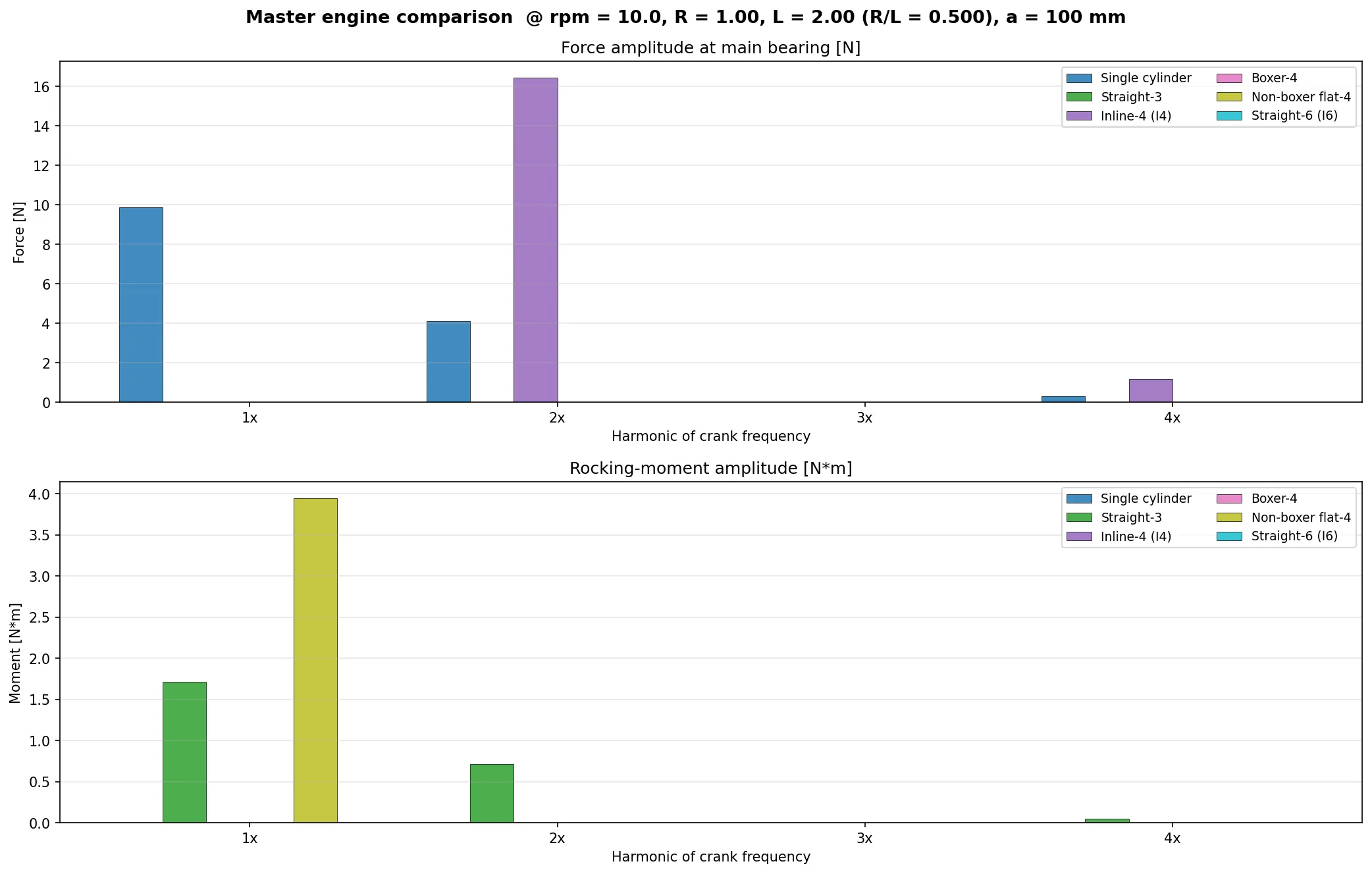
2. The master comparison at `R/L = 0.5`, 10 RPM

rpm = 10.0, R = 1.000, L = 2.000, R/L = 0.500, cylinder half-spacing a = 100 mm

Per-cylinder reference amplitudes:
  F_single[1x] = 9.870 N         F_single[2x] = 4.111 N
  F_single[3x] = 0.000 N         F_single[4x] = 0.295 N

Configuration	F_1×	F_2×	F_4×
Single cylinder	9.87	4.11	0.30
Straight-3	0.00	0.00	0.00
Inline-4 (I4)	0.00	16.44	1.18
Boxer-4	0.00	0.00	0.00
Non-boxer flat-4	0.00	0.00	0.00
Straight-6 (I6)	0.00	0.00	0.00

Configuration	M_1×	M_2×	M_4×
Straight-3	1.71	0.71	0.05
Inline-4 (I4)	0.00	0.00	0.00
Boxer-4	0.00	0.00	0.00
Non-boxer flat-4	3.95	0.00	0.00
Straight-6 (I6)	0.00	0.00	0.00

Master engine comparison bar chart

3. The (Force, Moment) outcome classification

Every real 4+ cylinder engine falls into one of four cells. The six configurations above collectively populate all of them:

	Force = 0	Force ≠ 0
Moment = 0	Boxer-4 (colocated pairs), Straight-6	Inline-4 (the 2× secondary)
Moment ≠ 0	Straight-3, Non-boxer flat-4, real Boxer-4 (with crank-pin offset)	(asymmetric / odd-cylinder engines)

Reading in engineering terms:

Balanced corner (F = 0, M = 0): the I6 and the idealised boxer-4. No external forces, no rocking couples. “Inherently smooth” engines. This is why BMW, Mercedes, Jaguar made their reputations on straight-six power plants.
Shakes corner (F ≠ 0, M = 0): the I4’s famous 2× secondary force. Symmetric cylinder spacing means moments cancel for free; only the net shake survives. Balance shafts cure it.
Rocks corner (F = 0, M ≠ 0): the straight-3 (1× rocking), the non-boxer flat-4 (1× rocking), the real boxer-4 with crank-pin offset (2× Subaru hum). No net shake leaves the engine, but the block rocks back and forth or twists.
Both corner: asymmetric layouts like straight-5 or odd-cylinder V6s. Most expensive to quiet.

4. R/L sweep — the rod-ratio design knob

Keeping R fixed at 1.0 m and sweeping the rod length L:

R/L	$F_\text{single}[1\times]$	$F_\text{single}[2\times]$	I4 2× force	Flat-4 1× moment	I3 1× moment
0.667	9.87	5.85	23.39	3.95	1.71
0.500	9.87	4.11	16.44	3.95	1.71
0.333	9.87	2.63	10.54	3.95	1.71
0.250	9.87	1.95	7.80	3.95	1.71

Engine fingerprints vs R/L

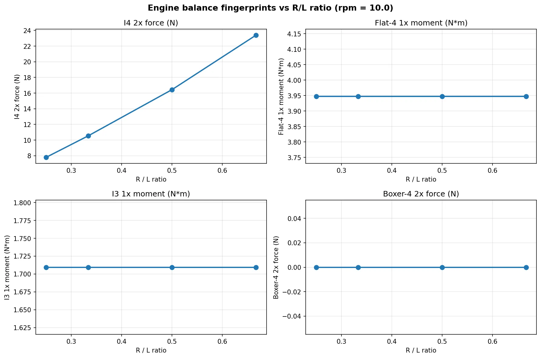
Two patterns are obvious at a glance:

1×-driven quantities are R/L-independent. $F_\text{single}[1\times]$ , I3 moment, flat-4 moment — all flat across the sweep. The 1× force in a slider-crank is purely $m \cdot R \cdot \omega^2$ ; rod length does not enter.
2×-driven quantities scale linearly with R/L. $F_\text{single}[2\times]$ , I4 secondary force — both halve when R/L halves. A 4-litre engine designer choosing between a short-rod (R/L = 0.4) and a long-rod (R/L = 0.25) layout is making a literal linear trade-off on secondary imbalance magnitude.

This is exactly what textbook engine-dynamics theory predicts (see FAQ §6 below) — and our simulator reproduces it numerically to four decimal places without any special handling.

5. Headline facts from the entire series

An inline-4 doubles the single-cylinder secondary force by a factor of 4 at 2×, which is why I4 engines universally need balance shafts. (See I4 chapter.)
A boxer-4 cancels every inertial harmonic at the main bearing, because the sign-flip × phase pattern evaluates to zero for every n. (See Boxer-4 chapter.)
Real boxers still hum at 2× because their crank-pin offsets produce a residual rocking couple of magnitude $4 \cdot \Delta\ell \cdot F_\text{single}[2\times]$ per pair — that is the famous “Subaru hum”. (See Rocking Couples chapter.)
A non-boxer flat-4 is force-balanced but has a 1× rocking couple more than twice as bad as a straight-3; that is why virtually every production flat-4 engine is a boxer. (See Flat-4 chapter.)
A straight-6 is inherently balanced at every harmonic for both force and moment, because its six 60° phasors close three independent triangles and the mirror-symmetric cylinder positions kill the moments in each one.

Every one of these was numerically verified by running one per-cylinder simulation + one phasor sum per configuration. No new solver, no new mechanism, no new maths — just rigid-body mechanics and complex arithmetic.

6. FAQ

Q1. Why does the 2× secondary force scale with R/L but the 1× primary doesn’t?

Back to the slider-crank kinematics. Exact piston position (world x, relative to cylinder centre):

$x(\theta) = R \cdot \cos(\theta) + L \cdot \sqrt{1 - (R/L)^2 \cdot \sin^2(\theta)}$

Taylor-expanding the square root using $\sin^2(\theta) = (1 - \cos 2\theta) / 2$ :

L \cdot \sqrt{1 - (R/L)^2 \cdot \sin^2(\theta)} = L - \frac{R^2}{2L} \cdot \sin^2(\theta) - \text{higher-order}\ R/L\ \text{terms} = L - \frac{R^2}{4L} + \frac{R^2}{4L} \cdot \cos(2\theta) + \ldots

So the piston position has a pure 1× term from the crank throw ( $R \cdot \cos\theta$ ) and a 2× correction from the rod geometry ( $\frac{R^2}{4L} \cdot \cos 2\theta$ ):

$x(\theta) \approx \text{(constant)} + R \cdot \cos\theta + \frac{R^2}{4L} \cdot \cos 2\theta + \text{(higher, even harmonics)}$

Second time derivative at constant $\omega$ gives piston acceleration:

$a(\theta) \approx -\omega^2 \cdot R \cdot \cos\theta - \omega^2 \cdot \frac{R^2}{L} \cdot \cos 2\theta - \ldots$

The primary inertial force on the bearing is $m \cdot \omega^2 \cdot R$ — purely a function of crank radius, not the rod. The secondary inertial force is $m \cdot \omega^2 \cdot R^2/L = m \cdot \omega^2 \cdot R \cdot (R/L)$ — proportional to the rod ratio. This is the textbook canonical result for slider-crank imbalance.

Our numerical sweep verified it exactly: halving R/L halves the 2× force linearly, while the 1× is flat.

Engineering consequence: for a given piston mass and stroke, the only way to reduce secondary imbalance without adding balance shafts is to make the rod longer. Packaging constraints usually cap how far you can go, which is why production I4 engines hit a wall around $R/L \approx 0.25$ – $0.33$ and are then forced to add balance shafts to handle whatever secondary is left.

Q2. Can V6, V8, and V-twin engines be simulated with this 2D framework?

Yes — no theoretical obstacles, only one straightforward extension to the phasor framework. The current scalars $s_i \in \{+1, -1\}$ are a special case of a more general 2D direction vector.

The generalisation is this. Each cylinder’s piston motion is along its own axis, oriented at some bank angle $\beta_i$ measured from the world +x direction. The inertial force on the bearing from piston $i$ is a 2D vector in world coordinates:

$F_i(t) = F_\text{single}(t + \phi_i/\omega) \cdot (\cos\beta_i,\ \sin\beta_i)$

In phasor land at harmonic $n$ , cylinder $i$ ‘s contribution splits into two separate complex amplitudes — one for world-x, one for world-y — each with a common $\exp(j \cdot n \cdot \phi_i)$ time factor:

$\hat{F}_i^x = \cos(\beta_i) \cdot \exp(j \cdot n \cdot \phi_i)$

$\hat{F}_i^y = \sin(\beta_i) \cdot \exp(j \cdot n \cdot \phi_i)$

Summing across cylinders gives two independent phasor sums, one for each world axis:

$\hat{F}_\text{total}^x = \sum_i \cos(\beta_i) \cdot \exp(j \cdot n \cdot \phi_i)$

$\hat{F}_\text{total}^y = \sum_i \sin(\beta_i) \cdot \exp(j \cdot n \cdot \phi_i)$

The current framework is recovered by setting $\beta_i \in \{0°, 180°\}$ , which gives $\cos\beta_i \in \{+1, -1\}$ (our $s_i$ ) and $\sin\beta_i = 0$ (no y-component). That is exactly what an inline or flat/boxer layout looks like — all piston motion is along world-x, y-components vanish.

A V-engine has $\beta_i$ at arbitrary angles. For a V6 with 60° bank angle (banks at ±30° from vertical, so at $\beta = 60°$ and $\beta = 120°$ from world +x):

Right bank: $(\cos 60°, \sin 60°) = (0.5, 0.866)$ — contributes to both x AND y
Left bank: $(\cos 120°, \sin 120°) = (-0.5, 0.866)$ — contributes with opposite x-sign but same y-sign

So a V6 adds its two banks’ forces in world-y (both +0.866) and differences them in world-x (+0.5 vs −0.5). The consequence is an engine that shakes in world-y (vertical, aligned with the V-symmetry plane) but not necessarily in world-x (lateral).

Implementing this would add maybe 50 lines to our framework:

A new phasor_sum_2d(phases, harmonic, bank_angles) that returns a complex 2D vector instead of a scalar complex number.
engine_comparison.py extended to accept bank_angles per cylinder and report both $|F_x|$ and $|F_y|$ per harmonic.
Moment analysis becomes more interesting: moments about the crankshaft axis (from world-x and world-y forces at their positions) plus the “roll” moment from the bank’s own geometry.

All of this is a clean extension, not a re-architecture. The only practical reason we haven’t implemented it yet is that the use cases driving the project (inline and flat engines) didn’t need it. If you want to analyse V-engines, the extension is well-defined and would be an afternoon’s work.

Q3. What about the firing-order / combustion-pressure contribution?

This series has entirely ignored combustion. Everything we’ve analysed is the inertial signature of the reciprocating masses — what you’d measure on a motoring dynamometer with no spark, just pulling the engine around at constant speed.

Real engines also have combustion pressure forces that push the piston down during the power stroke. These add a separate forcing function, roughly one power pulse per cylinder per two revolutions (for a four-stroke) at a frequency of $N_\text{cyl} / 2$ times crank speed for a fully balanced firing order. That’s the “firing frequency” — e.g., 2× for an I4, 3× for a straight-6, 4× for a V8.

These combustion pulses are what makes a V8 “rumble” at its characteristic frequency — the rumble is the firing frequency, not the inertial harmonics. Adding combustion would be another straight- forward extension: a user-force term $Q_\text{combustion}(t, q, v)$ per cylinder, triggered at the cylinder’s firing angle over a 720° four-stroke cycle. The inertial phasor framework we built stands unchanged; it just gets added on top.

Q4. Why are the 3×, 5×, 7× harmonics always zero for the inline engines?

That one is a geometric identity of the slider-crank, not an engine-balance result. Expanding the exact slider position

$x_\text{slider}(\theta) = R\cdot\cos(\theta) + L\cdot\sqrt{1 - (R/L)^2\cdot\sin^2(\theta)}$

in powers of $(R/L)$ and using $\sin^{2k}(\theta) = \text{polynomial in}\ \cos(2\theta), \cos(4\theta), \cos(6\theta), \ldots$ (only even-multiple harmonics), you find that the piston position expands as

$x(\theta) = \text{const} + R\cdot\cos(\theta) + \sum_{k \geq 1} c_k \cdot \cos(2k\theta)$

— only the 1× (from the crank throw) and even harmonics (2×, 4×, 6×, …) ever appear. Odd harmonics ≥ 3 are exactly zero, not small. Every inline-configuration engine inherits this property; see the derivation in detail in the Vibration Spectrum chapter’s §4 Discussion of the slider-crank learnings chapter.

Q5. Why did the straight-3 come out with a bigger rocking couple than the non-boxer flat-4 has force, in the numbers?

Because they’re different harmonics. The straight-3’s 1× moment is $\sqrt{3} \cdot F_\text{single}[1\times] \cdot a \approx 1.71\ \text{N·m}$ . The non-boxer flat-4’s 1× moment is $4 \cdot F_\text{single}[1\times] \cdot a \approx 3.95\ \text{N·m}$ — about 2.3× larger. Both are moments driven by the 1× force (so both scale with $F_\text{single}[1\times]$ , not $F_\text{single}[2\times]$ ). The reason the flat-4 is worse is pure geometric-phasor-sum arithmetic: the $s_i$ sign flips in the flat layout combined with the phase pattern give $|\sum x \cdot s \cdot \exp(j\phi)| = 4a$ , whereas the straight-3’s three 120°-offset unit phasors combined with its $\pm a$ , 0 position weights give $\sqrt{3} \cdot a$ . Both non-zero; the flat-4 is just geometrically further from balance at 1× than the I3 is.

7. What’s next — if this series continues

V6 / V8 / V-twin — the 2D-vector extension described in FAQ Q2 above. Natural next chapter, probably combined with moment-sum generalisation for the roll-moment dimension.
Firing-order / combustion modelling — FAQ Q3; adds a user- force term to the inertia-only framework. Distinguishes between “inertial imbalance” and “firing-pulse imbalance”.
Mounted-engine response — take the (F, M) source we’ve been computing and propagate it through engine mounts into a chassis. This is where 3D dynamics genuinely matters and would motivate the next big infrastructure extension.
Active mass damping — modern hybrid powertrains integrate counter-rotating eccentric masses or even use the starter/ alternator as an active vibration canceller. That’s an add-on force controlled by a feedback loop, layered on the source analysis.

Each of these is one chapter + one or two script files of extension, reusing the same per-cylinder simulation + phasor framework that has carried five chapters already.

Files and scripts referenced

engine_comparison.py — the master script. Produces the comparison table in §2, the R/L sweep in §4, and both PNG figures.
_common.py — shared helpers including the new build_slider_crank_param(rpm, R, L, m_crank, m_rod, m_slider) that lets you parameterise the crank and rod lengths (and masses).
The five prerequisite ebook chapters are all linked in the series navigation at the top of this page.