The Slider-Crank, Three Ways

Series: The Slider-Crank, Three Ways · Multi-Cylinder I4 → · Boxer-4 → · Rocking Couples → · Non-boxer Flat-4 → · Summary → · V-Engines → · Combustion → · Balance Shafts → · Engine Mounts → · Active Damping → · Chassis Response → · Engine Mounts →

Reference: Field Guide · Concepts Primer · Physics · Computational Machinery · Dimensional Reduction

A short field-guide to what happens when you drive a slider-crank at a constant speed and ask: what does the motor supply, what do the bearings feel, and what spectrum of vibrations comes out of the block? — first with gravity, then without, and why the comparison matters.

Built on the Python multibody toolkit in this repo. All numbers and figures come from real simulations; every claim you can re-run in a minute.

The mechanism

A single-cylinder slider-crank with realistic masses:

Body	Mass	Inertia	CG offset	Role
Ground	0	0	—	frame
Crank (L = 1 m)	2 kg	0.14 kg·m²	(0.5, 0) m	rotates
Connecting rod (L = 2 m)	4 kg	0.32 kg·m²	(0, 0)	crank → slider
Slider	5 kg	0.05 kg·m²	(0, 0)	reciprocates along x

Constraints: 3 revolute pairs (ground–crank, crank–rod, rod–slider) + 1 prismatic (slider on ground’s x-axis) + 1 user constraint $\theta_\text{crank} - \omega \cdot t = 0$ that drives the crank at 10 RPM.

With the user constraint locked, the mechanism is kinematically fully determined — n_coord = n_restr = 12, zero free DOFs. That is the setup where inverse dynamics makes sense.

Act 1 — Inverse dynamics: forces given motion

At every instant the solver forms the saddle-point system

\begin{bmatrix} \mathbf{M} & \mathbf{C}_q^T \\ \mathbf{C}_q & \mathbf{0} \end{bmatrix} \begin{bmatrix} \mathbf{a} \\ \boldsymbol{\lambda} \end{bmatrix} = \begin{bmatrix} \mathbf{Q}_\text{total} \\ \boldsymbol{\gamma} \end{bmatrix}

and reads off $\mathbf{a}$ (accelerations consistent with prescribed motion) and — crucially — $\boldsymbol{\lambda}$ , the Lagrange multipliers. These are the constraint reaction forces:

$\boldsymbol{\lambda}$ for a revolute joint = $(R_x, R_y)$ bearing reaction pair
$\boldsymbol{\lambda}$ for a prismatic joint = (angular moment, normal reaction)
$\boldsymbol{\lambda}$ for the driving user constraint = $-\tau_\text{driving}$ (sign convention)

No time integration: one linear solve per time step. For our 10 RPM slider-crank at 360 steps over 2 revolutions, it runs instantly.

The torque signature — a polar plot

The most memorable picture is $|\tau(\theta)|$ in polar coordinates — the motor’s “breathing pattern” over one rev.

Polar driving-torque, gravity ON

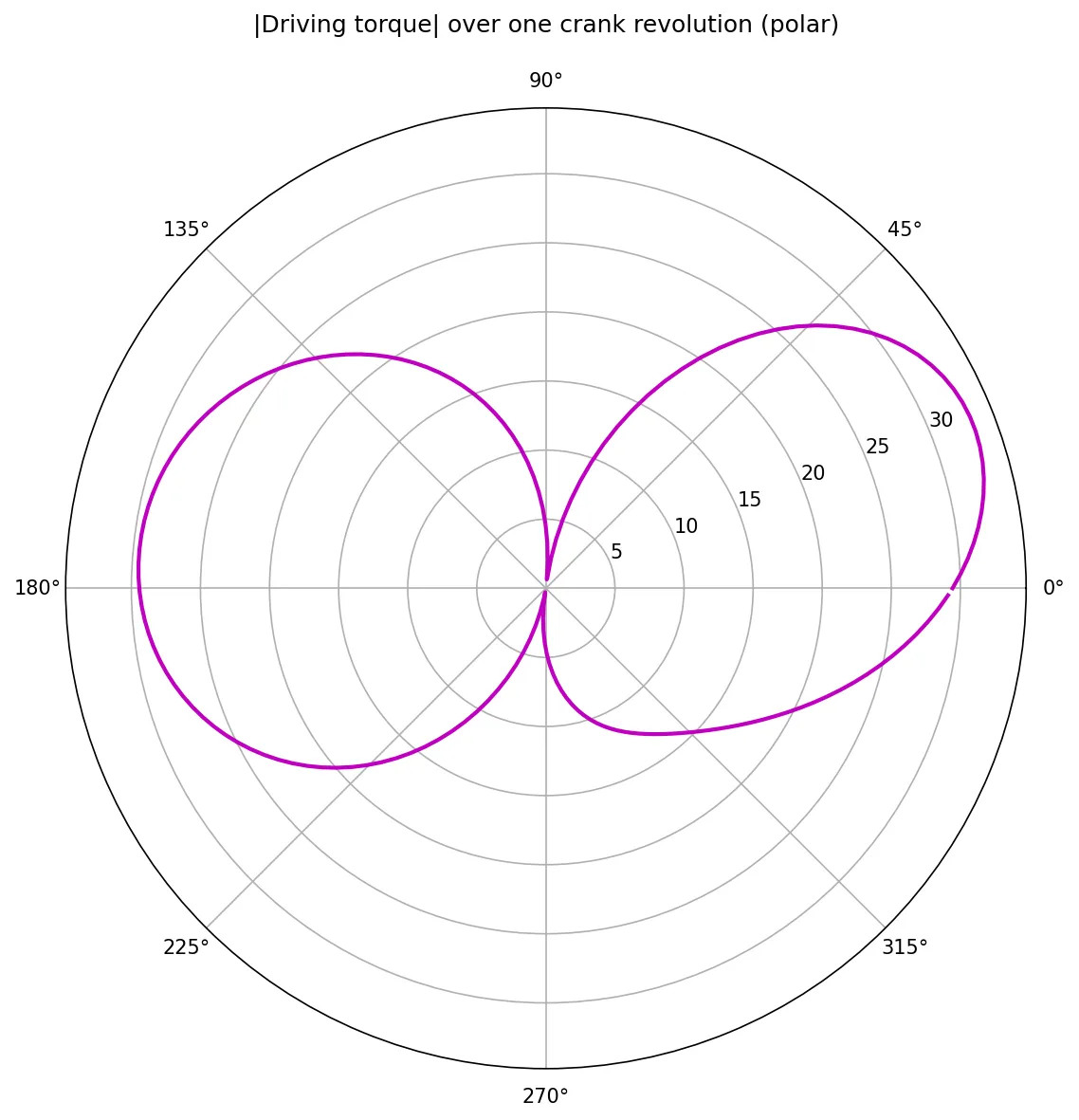
Two lobes, visibly asymmetric. The two lobes come from slider inertia reversing twice per revolution (at top- and bottom-dead-centre). The asymmetry is gravity tilting the response — the crank’s CG is offset $0.5\text{ m}$ from its pivot, so gravity adds a once-per-revolution sinusoid on top of the inertial response.

The time histories

Alongside the polar view, the same simulation gives the full trajectory of every reaction force over the cycle:

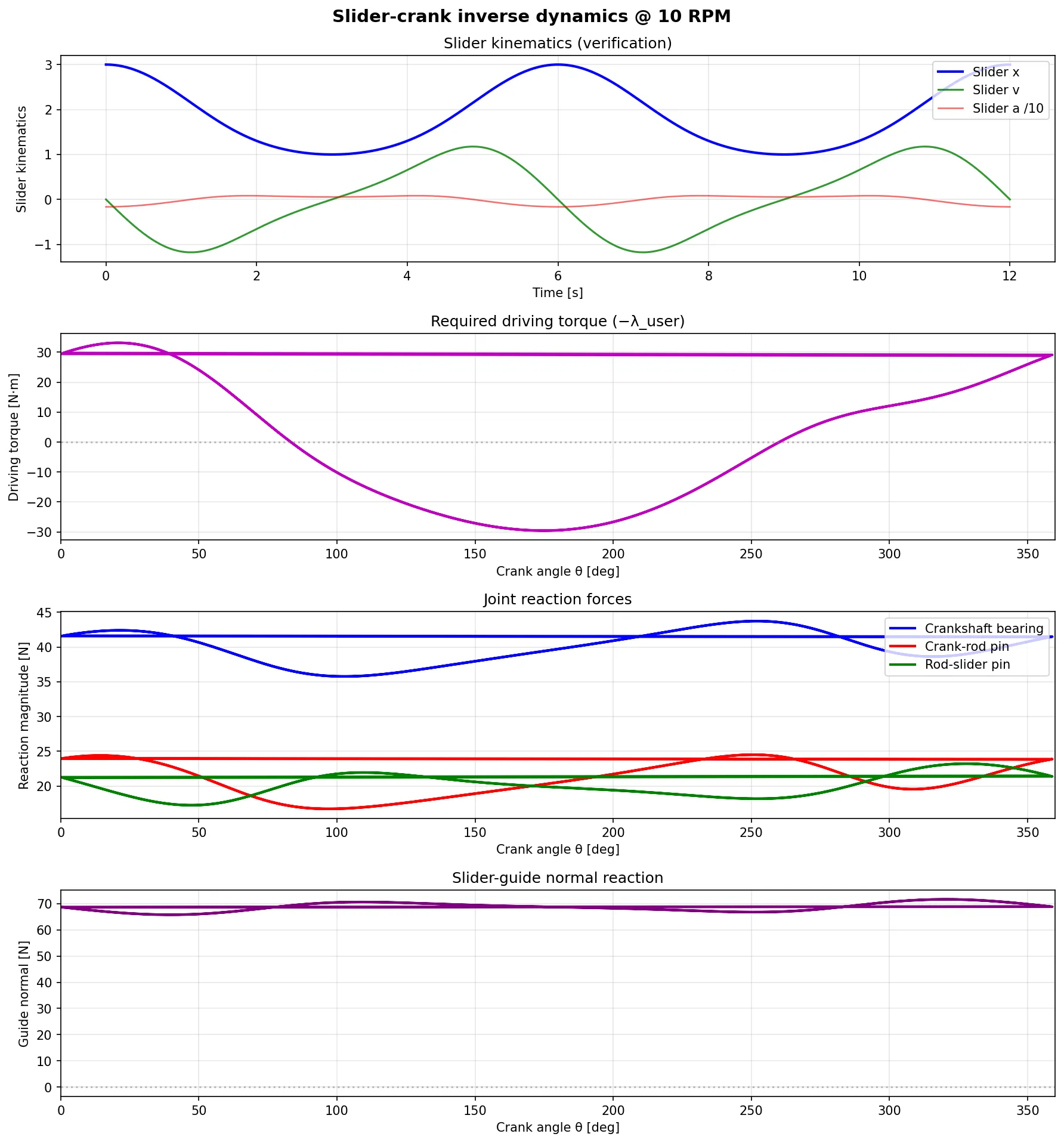
Inverse-dynamics overview, gravity ON

From top to bottom:

Slider kinematics — verification that the slider actually moves the way it should (stroke 1 → 3 m, two dead-centres per rev).
Driving torque vs crank angle — peak 33 N·m. That’s the number that sizes the motor.
Bearing-reaction magnitudes — three colored traces for the three pins (crankshaft bearing, crank-rod, rod-slider). Peak 44 N at the crankshaft bearing.
Slider-guide normal — peak 72 N. Most of this is just the slider’s weight being supported; only a few N is dynamic.

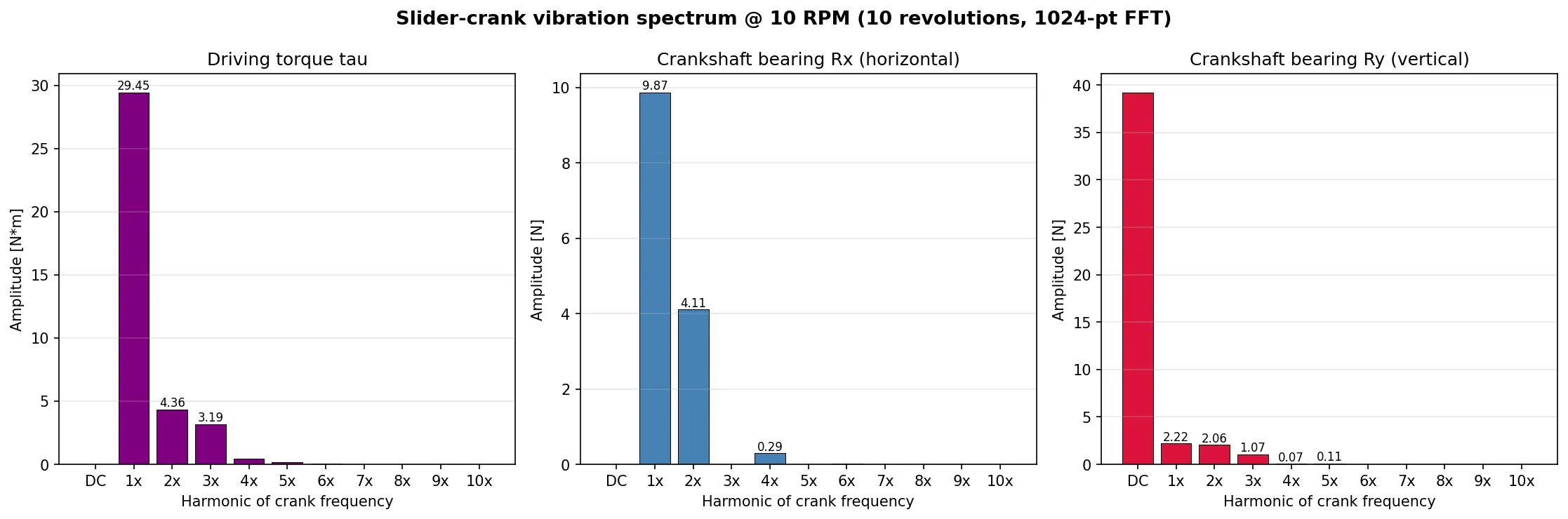
Act 2 — Vibrations: what the FFT reveals

A mechanism running at constant RPM is periodic. Any time-domain signal — torque, force, penetration — can be decomposed into harmonics of the crank frequency. We run the same mechanism for 10 full revolutions, FFT $\tau(t)$ , $R_x(t)$ , and $R_y(t)$ , and read off the amplitudes at 0×, 1×, 2×, …, 10×.

Vibration spectrum, gravity ON

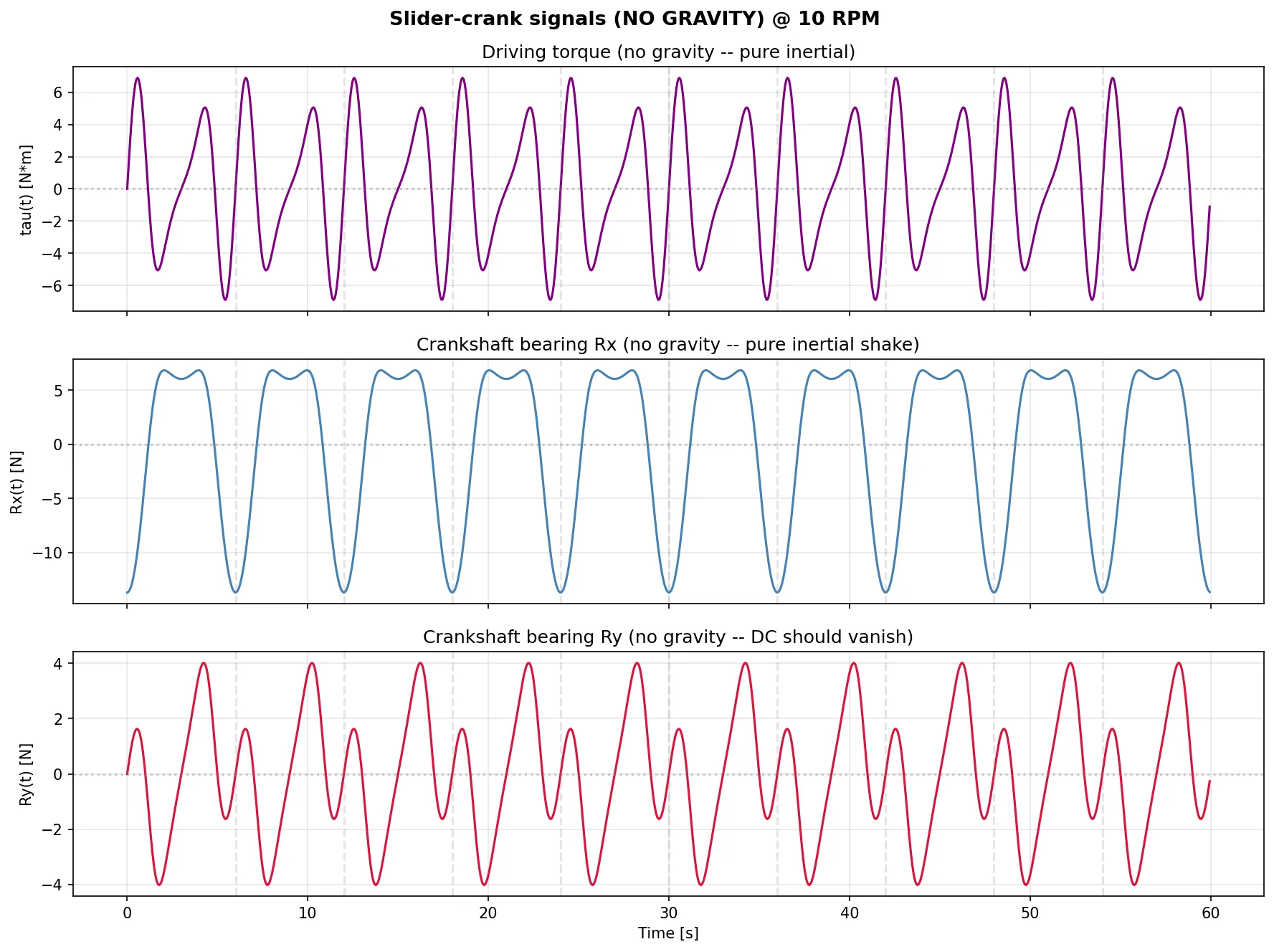
The same data, as a time-history, with revolution boundaries marked:

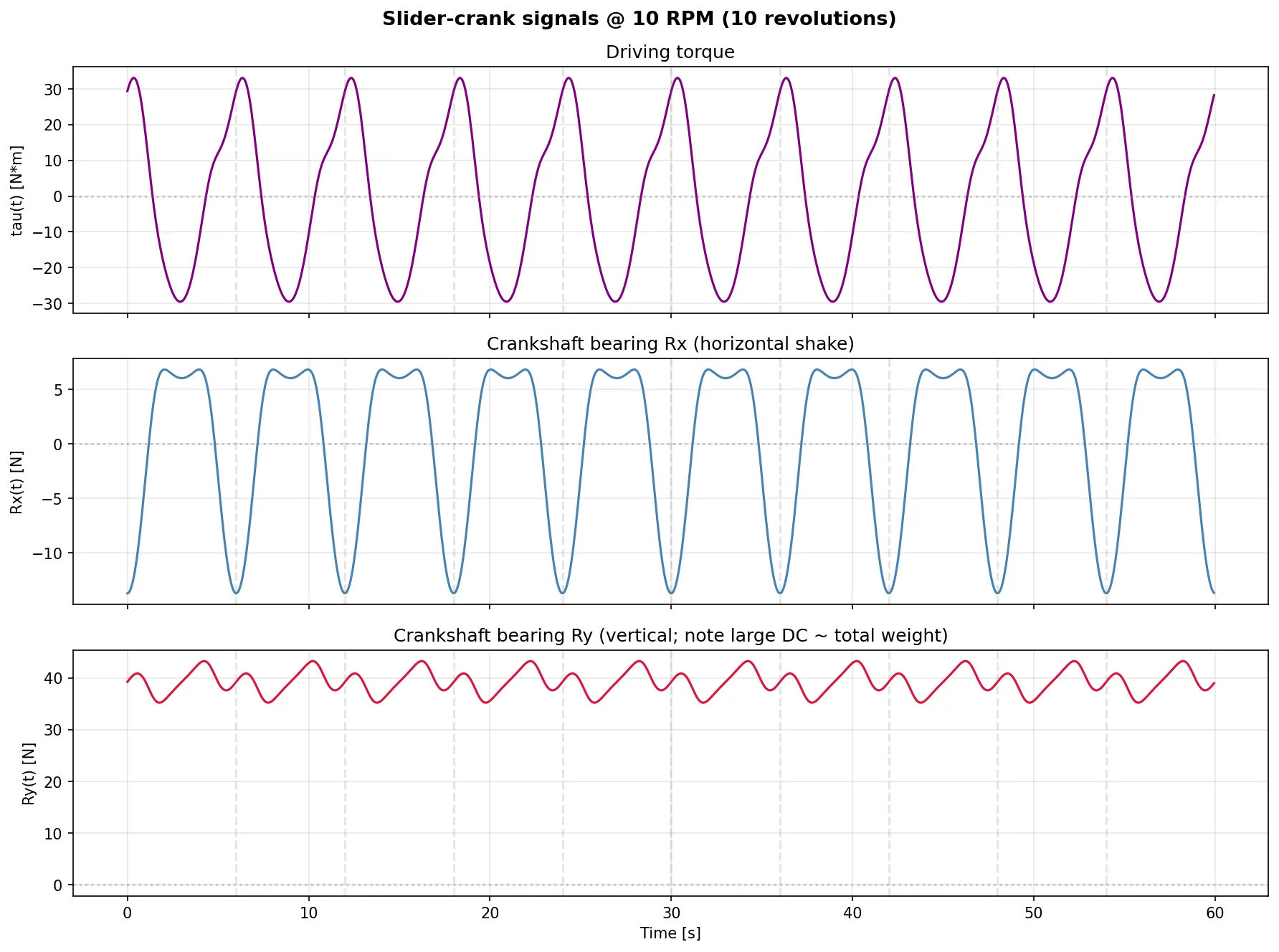
Vibration time histories, gravity ON

Three facts jump out of the spectrum:

1. DC $R_y = (m_\text{crank} + m_\text{rod}/2) \cdot g$ exactly

Measured: 39.24 N, matching $2g + 2g = 4g = 39.24$ on the nose. Why? Under gravity, the crankshaft bearing supports the crank’s own weight plus half of the rod’s weight (the rod is symmetric with CG at its centre, so it shares its weight 50/50 between its two pins). The slider’s weight goes to the guide, not the bearing.

If you build your own mechanism and the DC bearing reaction doesn’t match this kind of hand-check, you’ve mis-specified a mass somewhere — this is the cheapest sanity check in all of multibody dynamics.

2. Odd harmonics (≥ 3) of $R_x$ vanish exactly

$R_x[3\times] = R_x[5\times] = R_x[7\times] = 0$ , to numerical precision. This isn’t an approximation — it’s a rigorous identity from the slider-crank kinematics. Taylor-expanding the slider position

$x_\text{slider}(\theta) = R\cos\theta + L\sqrt{1 - (R/L)^2 \sin^2\theta}$

using $\sin^2\theta = (1 - \cos 2\theta)/2$ and $\sin^4\theta$ expressed in $\cos(2\theta)$ and $\cos(4\theta)$ terms, you find the square root contributes only even cosine harmonics (2×, 4×, 6×, …) on top of the exact 1× term from $R\cos\theta$ . No 3×, 5×, 7× ever appear.

Consequence: a single-piston engine cannot emit mechanical shake at 3× crank frequency through the block-mount pathway. If you measure 3× noise on a real engine, it has to come from somewhere else — the valvetrain, combustion pressure waves, bearing defects.

3. Secondary imbalance is 4.11 N at 2×

Measured: $R_x[2\times] = 4.11\text{ N}$ . First-principles prediction from the expansion above:

$F_2 \approx m_\text{slider} \cdot \omega^2 \cdot R^2 / L = 5 \cdot 1.047^2 \cdot 1 / 2 = 2.74\text{ N}$

We measured 4.11 N — the extra ~1.4 N comes from the rod’s own 2× inertia (the rod CG oscillates too, with its own even-harmonic content). Order-of-magnitude: correct.

This is the number that sizes balance shafts. In a 4-cylinder inline engine, the 1× components from the four pistons cancel exactly (180°-paired), but the 2× components all add up in phase (180° × 2 = 360° = in phase). So an I4 has 4× this secondary imbalance force. That’s why Mitsubishi invented the Silent Shaft and why every modern 2-litre 4-cylinder has a pair of balance shafts turning at 2× crank speed.

Act 3 — The gravity-isolation experiment

The gravity-ON run couples two different physical effects:

Inertia — the masses of the crank, rod, and slider must be accelerated through their respective motions.
Gravity — each body with mass has a constant vertical force at its CG; any CG offset (the crank’s 0.5 m) turns this into a once-per-revolution torque.

To separate them, we run the exact same simulation with mb.g = np.array([0.0, 0.0]). One line of code, profound results:

Gravity-OFF spectrum side-by-side

No-gravity time histories

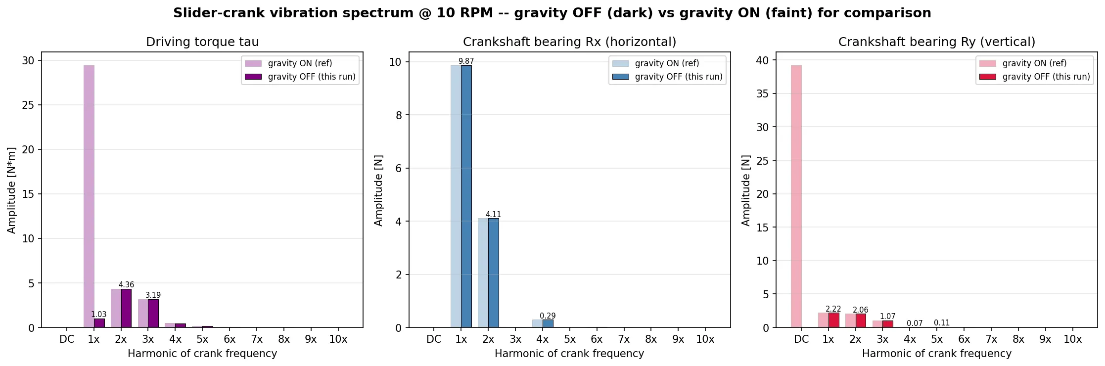
Here is the comparison table, the heart of this experiment:

Signal × harmonic	Gravity ON	Gravity OFF	Status
DC $R_y$	39.24 N	0.00 N	static weight, gone
1× $\tau$	29.45 N·m	1.03 N·m	mostly gravity — the ~29 N·m was the $m \cdot g \cdot d \cdot \cos\theta$ torque on the offset crank CG
1× $R_x$	9.87 N	9.87 N	identical — pure inertia, gravity-independent
2× $R_x$	4.11 N	4.11 N	inertial secondary, frame-invariant
Odd ≥ 3 $R_x$	0	0	geometric symmetry, always

This table deserves a moment. Notice what does and doesn’t change:

The 1× of $R_x$ is unchanged. That’s because our slider moves horizontally and gravity points vertically — orthogonal. Gravity cannot inject any horizontal component at any harmonic in this layout. All 9.87 N of primary shake force is pure inertia:

$1\times R_x \approx \omega^2 \cdot R \cdot (m_\text{slider} + m_\text{rod} + \tfrac{1}{2} m_\text{crank}) \cdot \cos\theta \approx 11\text{ N}$

(measured 9.87, with ~10% lost to higher-order rod corrections).
The 1× of $\tau$ collapses. It was 97% gravity. The once-per-rev sinusoid from the crank’s offset CG moving through the gravity field was the overwhelming share of the driving-torque ripple.
The slider-guide normal collapses from 72 N to 3 N. Almost all of it was static weight, dynamic content is minimal.
The 2× content is invariant. Mass distribution and geometry set it; orientation doesn’t matter.

The no-gravity polar plot

The torque signature without gravity is visibly different:

Polar torque, gravity OFF

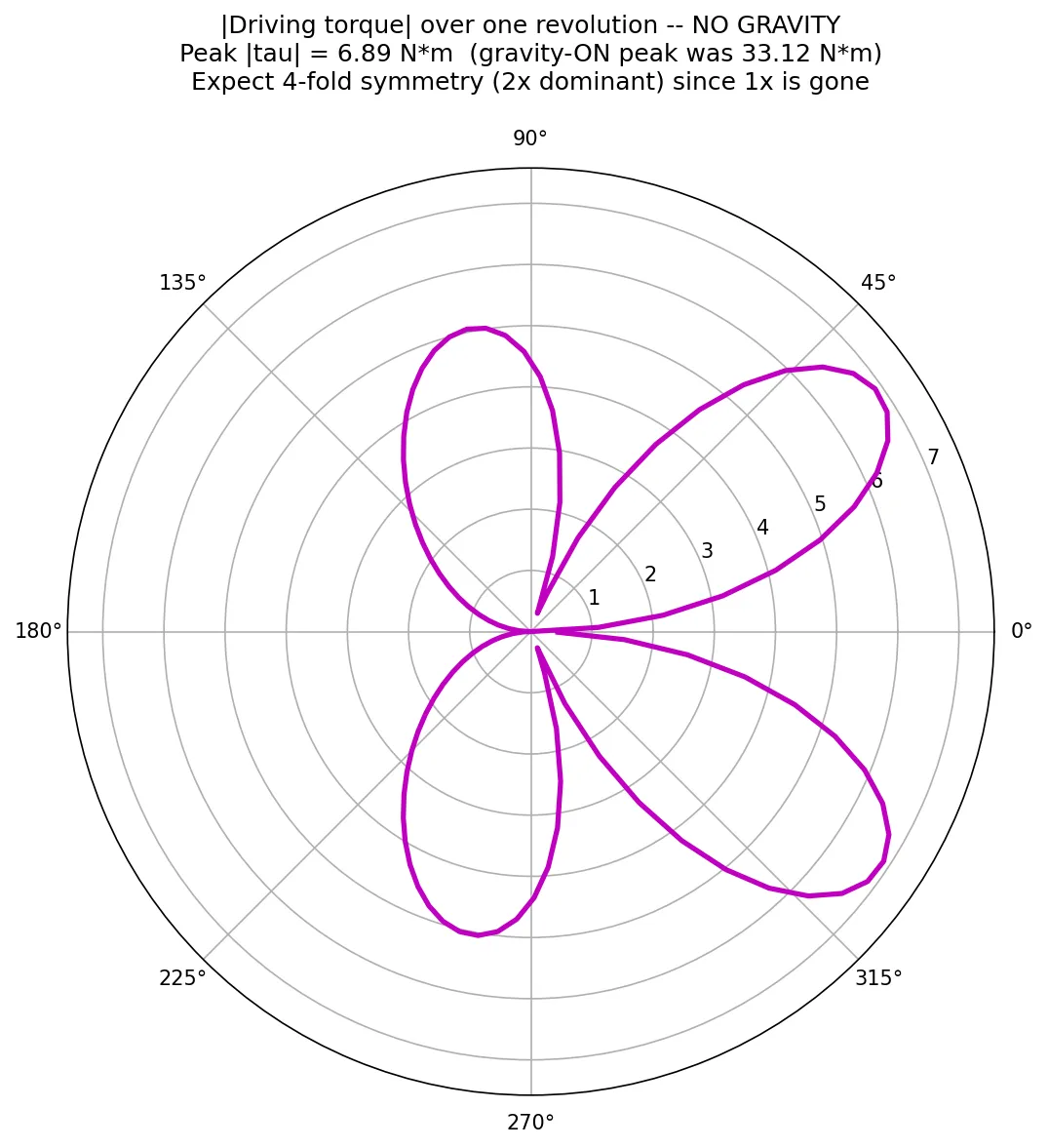
Four-fold (nearly) symmetric, peak only ~7 N·m (vs 33 N·m with gravity). The 2× harmonic dominates, so the shape approaches a four-lobe rose — the geometric fingerprint of pure inertial torque without gravity bias.

The no-gravity force-trend plot

Forces vs crank angle, gravity OFF

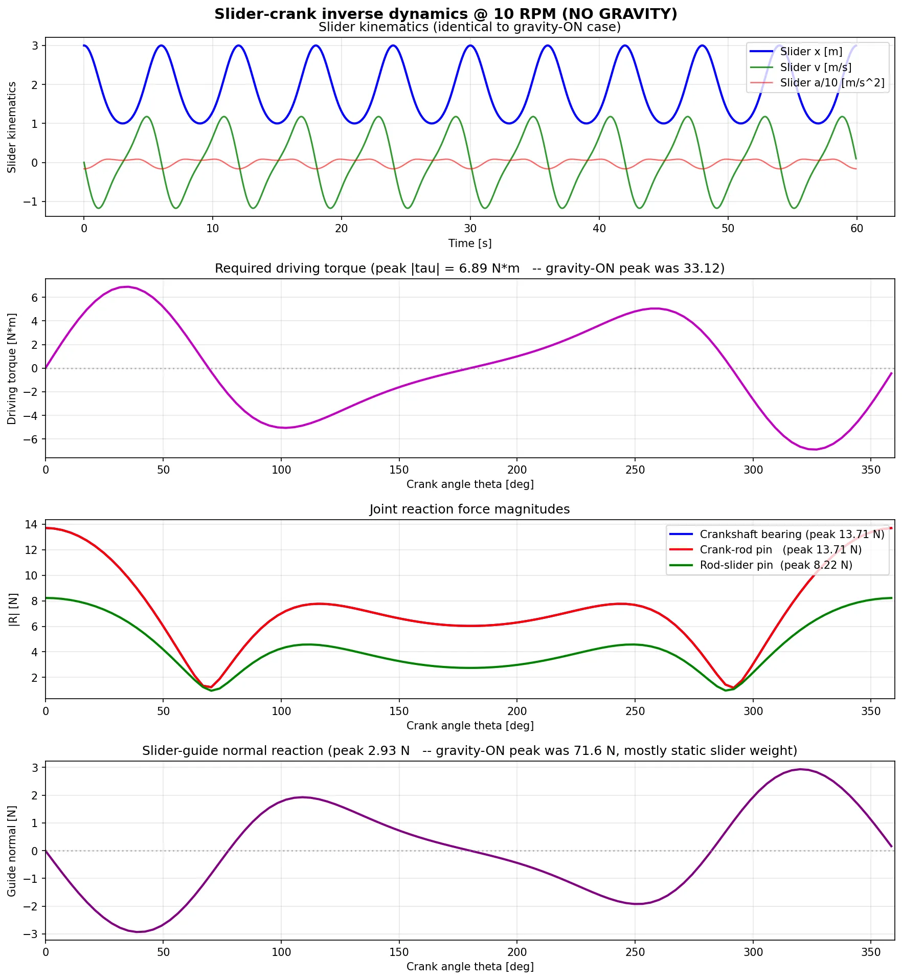
Side-by-side with the gravity-ON version, you see exactly which peaks were carrying static weight and which were dynamic. The slider-guide normal is the most dramatic change: from a 72 N peak dominated by static support, down to a 3 N dynamic ripple.

Layout matters for multi-cylinder analysis

The fact that in our horizontal layout gravity never injects horizontal shake force is layout-specific, and it matters for what comes next:

A vertical in-line cylinder (cylinder axis = piston travel axis = vertical) has gravity parallel to slider motion. The 1× of the along-piston bearing force picks up a gravity term; the perpendicular axis stays gravity-clean.
A horizontally-opposed (boxer) configuration has cylinders at 180° on opposite sides — gravity is perpendicular to both piston axes. Different from a flat-4 where pistons move in the same plane but aren’t mirrored.
An inline-4 has all pistons vertical in the same plane, driven by the same crankshaft with 180° phase offsets. The 1× cancellation is gravity-assisted in one axis and gravity-hostile in the other.

The next chapter in this progression — multi-cylinder superposition — is a phasing-and-summation exercise on top of the spectra we measured here. Each cylinder contributes the same per-cylinder spectrum (1× $R_x$ , 2× $R_x$ , …) but with a crank-phase offset. The firing order sets the relative phases. Harmonics that are in phase add constructively (engine shakes at that frequency); harmonics 180° out of phase cancel. The 2× always adds for any firing pattern that uses the 4-stroke cycle in a balanced way — which is why balance shafts are universal.

Takeaways

Inverse dynamics reveals everything about constant-speed operation: torque, bearing reactions, guide loads — no integration needed, one linear solve per time step.
FFT the signals to get the vibration spectrum. Harmonic decomposition is the bridge between multibody dynamics and classical NVH analysis.
DC reactions must match static hand-calculation — cheapest possible sanity check on a multibody model.
Odd harmonics ≥ 3 vanish from the horizontal force of a slider-crank. It’s a geometric identity, not an accident.
Gravity vs inertia cleanly decompose by toggling mb.g = [0,0]. Run both versions of every mechanism you care about; the difference is always more illuminating than either one alone.

Files and scripts referenced

All figures above were generated by:

inverse_slider_crank.py — the 4-panel overview and the polar plot (gravity ON)
vibration_slider_crank.py — the spectrum bar chart and time histories (gravity ON)
vibration_slider_crank_no_gravity.py — all four no-gravity plots

Supporting solver infrastructure:

solve_inverse_dynamics() — the workhorse; one saddle-point solve per time step
2d-slidercrank-inverse-learnings.md — detailed learnings for the polar plot + gravity decomposition
vibration_slider_crank.md — FFT-focused learnings, primary/secondary imbalance derivation, odd-harmonic identity proof