Engine-Mount Transmissibility — From Source to Chassis

Series: ← The Slider-Crank, Three Ways · ← Multi-Cylinder I4 · ← Boxer-4 · ← Rocking Couples · ← Non-boxer Flat-4 · ← Summary · ← V-Engines · ← Combustion · ← Balance Shafts · Engine Mounts · Active Damping → · Chassis Response →

Reference: Field Guide · Concepts Primer · Physics · Computational Machinery · Dimensional Reduction

Every chapter so far has stayed inside the engine, characterising the source — per-harmonic forces and moments imposed on the engine block by the cylinders. This chapter takes the source out: through the engine mounts to the chassis, and ultimately to the driver’s seat. That is the path NVH (noise, vibration, harshness) is judged on, and it is where the soft-vs-stiff mount tradeoff that every car manufacturer wrestles with actually lives.

The script: engine_mount_transmissibility.py.

1. The mount problem in one sentence

Engine mounts have two jobs that pull in opposite directions:

HOLD the engine still relative to the chassis (no wandering under torque, no contact with surrounding panels under shock load).
ISOLATE the chassis from engine vibration (no buzzing through the steering wheel, no booming in the cabin).

The first job wants the mounts stiff. The second wants them soft. Production engineering picks a single number that balances both, and lives with the consequences. This chapter quantifies what each choice does — numerically, harmonic by harmonic, across the RPM range.

2. The textbook 1-DOF result

The simplest model: engine mass $M$ on a spring $K$ with damping $C$ , forced by $F_0\cdot\cos(\omega\cdot t)$ . The force the mount transmits to ground is

$F_\text{chassis}(t) = K\cdot x(t) + C\cdot\dot{x}(t)$

In steady state, the transmissibility ratio is

$T(r, \zeta) = \frac{\sqrt{1 + (2\zeta r)^2}}{\sqrt{(1 - r^2)^2 + (2\zeta r)^2}}$

with $r = \omega / \omega_n$ (frequency ratio) and $\zeta = C / (2\sqrt{MK})$ (damping ratio). Three regions:

$r$	$T$	Interpretation
$r \ll 1$	$\approx 1$	Quasi-static. The mount just transmits the force; spring barely deflects.
$r \approx 1$	up to several	Resonance. Low damping → catastrophic amplification.
$r = \sqrt{2}$	exactly 1	Crossover.
$r \gg 1$	falls as $1/r^2$	Isolation. Inertia dominates; very little reaches the chassis.

1-DOF transmissibility curves

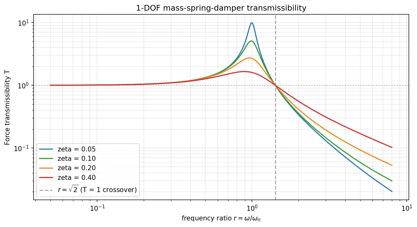
Two design principles fall out of this single curve:

Always operate above $r = \sqrt{2}$ . Below $\sqrt{2}$ the mount makes vibration worse, not better. Engine designers pick mount natural frequency $\omega_n$ such that the lowest excitation harmonic of interest sits well above $\sqrt{2}\cdot\omega_n$ .
Damping helps at resonance and hurts at isolation. High $\zeta$ tames the resonance peak but flattens the high-frequency rolloff (the $1/r^2$ becomes more like $1/r$ for very high $\zeta$ ). Production rubber mounts run $\zeta \approx 0.05$ – $0.15$ ; hydraulic mounts achieve a frequency-dependent $\zeta(\omega)$ that is high near resonance and low at high frequency. Both is the goal; either alone is a compromise.

3. The 3-DOF planar block

A real engine block has more than one DOF and more than one mount point. In the (x, y) cross-section perpendicular to the crankshaft — the working plane established in the Dimensional Reduction chapter — the block is a rigid body with three in-plane DOF:

$\mathbf{q} = (x_\text{block},\ y_\text{block},\ \theta_{z,\text{block}})$

It is excited by the source phasors $(\hat{F}_x, \hat{F}_y, \hat{M}_z)$ that the V-engine, combustion, and balance-shaft chapters already compute. ( $M_z$ is $M_\text{roll}$ , the engine output torque; in the in-plane working plane it’s the only moment that can excite block motion. $M_\text{pitch}$ and $M_\text{yaw}$ are out-of-plane moments here — see FAQ Q2.)

A mount at position $(x_m, y_m)$ relative to the block CG sees block displacement

$\delta_x = x_\text{block} - y_m \cdot \theta_z$

$\delta_y = y_\text{block} + x_m \cdot \theta_z \qquad \text{(small}\ \theta\ \text{approximation)}$

and applies forces $-k_x\cdot\delta_x$ and $-k_y\cdot\delta_y$ on the block, plus their moment about the CG. Collecting all that into a 3×3 stiffness matrix per mount (and damping matrix similarly), the equation of motion in the frequency domain is

$\left(-\omega^2 [\mathbf{M}] + j\omega [\mathbf{C}] + [\mathbf{K}]\right) \cdot \hat{\mathbf{q}} = \hat{\mathbf{F}}$

Solve this complex 3×3 linear system at each $\omega$ , sum the mount reactions to get the chassis-side force phasor, take the ratio with the source — that’s transmissibility per harmonic. The implementation is ~50 lines in engine_mount_transmissibility.py, no new infrastructure.

4. The soft-vs-stiff tradeoff for an I4

A representative 2 L transverse-mounted I4 on three mounts:

Parameter	Value
Block mass $M$	150 kg
Block inertia $I_z$	4 kg·m²
Mount positions (x, y) m, relative to CG	(+0.30, −0.10), (−0.30, −0.10), (0, +0.20)
Damping ratio $\zeta$ (rubber)	0.10
Soft mount: y-natural-frequency	8 Hz (typical road car)
Stiff mount: y-natural-frequency	25 Hz (sport car / truck)

Sweeping engine RPM from 500 to 6500 and reading transmissibility for the 2× crank harmonic (the dominant inertial + combustion frequency for an I4):

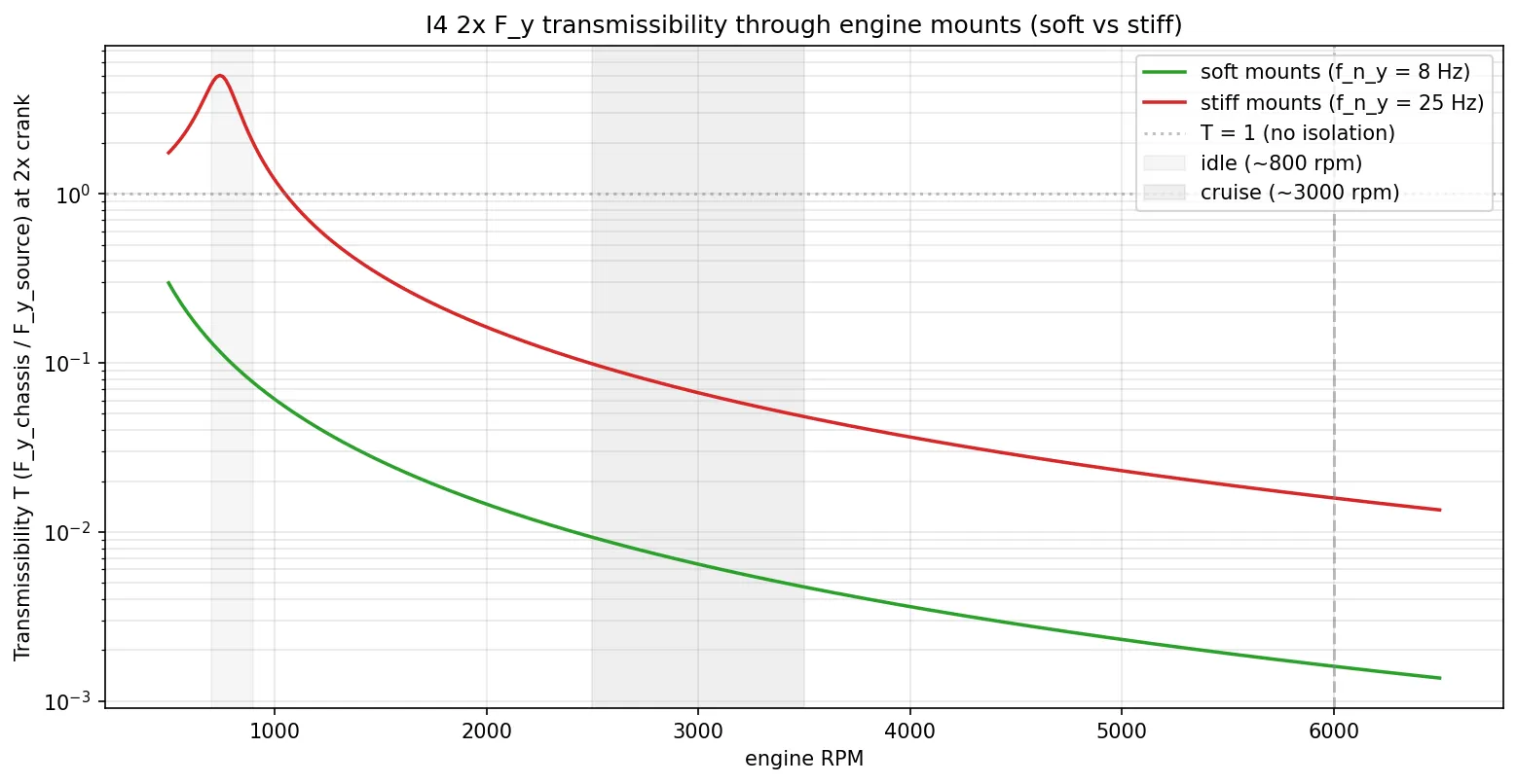
I4 2× transmissibility soft vs stiff

RPM	2× freq (Hz)	T (soft, 8 Hz)	T (stiff, 25 Hz)
500	16.7	0.30	1.75
800 (idle)	26.7	0.10	3.94 ← stiff resonance
1500	50.0	0.026	0.33
3000 (cruise)	100.0	0.0064	0.067
4500	150.0	0.0029	0.029
6000 (redline)	200.0	0.0016	0.016

Three things jump out of this table:

4.1 Stiff mounts resonate at idle

The 25 Hz mount has its natural frequency inside the engine’s idle range. At 800 RPM, 2× crank lands almost exactly on it — $r \approx 1.07$ — and the mount amplifies the source by a factor of nearly 4 instead of isolating. This is the cabin “boom” that owners of older sport cars and trucks know intimately. Production cars almost never allow this geometry.

4.2 Soft mounts win at cruise by an order of magnitude

At 3000 RPM, soft mounts let through 0.6% of the source, stiff mounts 6.7%. Same source, same RPM, same engine — one mount choice gives 10× better isolation. This is why every road car since 1990 uses $\omega_{n,y}$ in the 5–10 Hz range.

4.3 The high-RPM tail is the same on both, in shape

Both curves fall as $1/r^2$ at high frequency — that is just the inertia term in the EOM dominating both stiffness and damping. The absolute level is set by $1/k$ , so soft mounts always win at high frequency. The ratio between the two curves is constant ≈ 10× above ~80 Hz.

5. The concrete chassis force at 3000 RPM

Plugging in representative numbers for a real 2 L I4 at moderate load:

Source 2x at 3000 RPM (= 100 Hz):
    inertial    F_y =  2400 N        (4 cyl × m·ω²·R²/L)
    combustion  F_y =  5000 N        (firing-frequency beat)
    total       F_y =  7400 N

Through the mounts:

Mount choice	Block displacement \|y\|	Chassis force \|F_y\|	T
Soft (8 Hz)	0.126 mm	47.7 N	0.0064
Stiff (25 Hz)	0.133 mm	492.6 N	0.0666

Two observations worth pausing on.

Block displacement is nearly identical for both mount choices. That’s not an accident: at 100 Hz on a 150 kg block, the inertia term $\omega^2\cdot M \approx 5.9\ \text{MN/m}$ dwarfs the soft-mount stiffness (0.5 MN/m total) and even substantially exceeds the stiff-mount stiffness (4.9 MN/m). So $q \approx F/(\omega^2\cdot M)$ regardless of mount, giving the same ~0.13 mm engine motion. Engine motion is set by inertia above resonance, not by mount stiffness.

Chassis force differs by 10×. Same engine motion, different spring → $F_\text{chassis} = k \cdot q$ scales with mount stiffness. The whole point of going soft is to make $k$ small and reduce the spring force, not to reduce engine motion (which is set by inertia anyway). This is the cleanest mental model of mount design at typical operating frequencies.

6. Why soft mounts can’t be infinitely soft

The transmissibility math says softer is always better at operating frequency. Three constraints stop you from going to zero:

6.1 Static deflection from gravity

A 150 kg engine on $f_n = 1\ \text{Hz}$ mounts would sag by

$\delta_\text{static} = \frac{g}{(2\pi f_n)^2} = \frac{9.81}{39.5} \approx 25\ \text{cm}$

just from its own weight. Production engine bays do not have 25 cm of vertical clearance. Even at 5 Hz the static sag is 1 cm, which already complicates exhaust-pipe routing and the engine-to-trans mating. 8–10 Hz keeps static deflection at 2.5–4 mm, manageable.

6.2 Shock loads

A pothole or hard braking applies transient g-loads to the engine through the chassis (in reverse: chassis accelerates, engine on its mount swings back). Mount displacement under a shock scales as $F/k = F\cdot\delta_\text{static}/(M\cdot g) \propto 1/f_n^2$ . Halve $f_n$ , quadruple the shock excursion. Soft mounts hit clearance bumpers under road events; bumpers are ugly and add nonlinearity.

6.3 Engine roll under torque

The harmonic ripple of $M_\text{roll}$ (engine output torque) excites the $\theta_z$ DOF. With low $\omega_n$ for the rotational mode the engine rolls visibly on its mounts during throttle transients — the satisfying “V8 blip lurch”, desirable in a muscle car, undesirable in a luxury sedan where the same effect translates to a tip-in jerk in the cabin. The 3-DOF model captures this directly: solve with $\hat{\mathbf{F}} = (0, 0, \hat{M}_z)$ and read off $\theta_{z,\text{block}}$ .

Production sweet spot: $f_{n,y} \approx 8$ – $12\ \text{Hz}$ , $f_{n,x}$ slightly lower, $f_{n,\theta}$ (roll) tuned per-application — stiffer for sport cars, softer for luxury — typically 12–18 Hz.

7. Hydraulic and active mounts

Two upgrades from the linear constant-stiffness model:

Hydraulic mounts

A rubber mount with a fluid-filled chamber and a flow restriction between two cells. At low frequency the fluid sloshes through the restriction, providing high damping that tames the resonance peak. At high frequency the fluid can’t slosh fast enough; the mount behaves like a low-damping rubber mount, providing good isolation. Effectively you get $\zeta_\text{low} \approx 0.4$ – $0.5$ near $f_n$ and $\zeta_\text{high} \approx 0.05$ at cruise — the best of both regions on the 1-DOF chart.

In the framework: replace the constant $c$ in the damping matrix with a frequency-dependent $c(\omega)$ . The 3×3 solve at each $\omega$ already handles it; the math doesn’t notice.

Active mounts

An electromagnetic actuator inside (or replacing) the mount. Reads chassis-side acceleration with a sensor, computes an opposing force, drives the actuator. In principle achieves $T \approx 0$ at the target frequency.

Practical implementation: cancel just the firing-frequency component (the loudest single harmonic), leave the rest to passive isolation. Mercedes, Lexus, and the Audi S8 V10 used this approach in the 2000s to deliver V8/V10 character with no idle vibration in the cabin.

In the framework: an active mount is an extra phasor source term in $\hat{\mathbf{F}}$ whose magnitude and phase depend on the chassis-side measurement — i.e., a feedback loop on the existing linear model. The engineering question becomes a control-systems question (loop stability, sensor noise, actuator delay), but the underlying transmissibility math is unchanged.

8. FAQ

Q1. The 1-DOF and 3-DOF results look identical for pure F_y excitation. Why bother with 3-DOF?

For a symmetric mount layout with the source force aligned with the CG, the 3-DOF system decouples: y-translation is independent of x and $\theta$ . So pure $F_y$ excitation gives 1-DOF dynamics. The 3-DOF model becomes essential when:

The source has multiple components ( $F_x$ , $F_y$ , $M_z$ together) — they cross-couple via mount geometry, especially when the layout is asymmetric (top mount offset from CG).
Mount layout is asymmetric — a transverse-mounted I4 on a body-mount + torque rod has the torque rod doing most of the $M_\text{roll}$ reaction while the body mounts handle $F_y$ . The 1-DOF reduction lies about that.
The roll DOF is excited by $M_\text{roll}$ harmonic ripple.

For honest analysis of any production engine layout, 3-DOF is the minimum. We showed the symmetric $F_y$ case here because it makes the soft-vs-stiff story easy to read; the script supports any combination.

Q2. What about M_pitch and M_yaw from the V-engine chapter? Where do they go?

Those moments are about the y- and x-axes, out of the in-plane working plane for our 2D framework. The 3-DOF planar mount model in this chapter cannot propagate them in this cross-section; you’d need either a separate 2D analysis in the (x, z) side-view plane (where $M_\text{pitch}$ becomes the in-plane moment about z’) or a full 6-DOF 3D mount model. The same dimensional-reduction logic applies — see the Dimensional Reduction chapter §7 and §8.

In production NVH practice, $M_\text{pitch}$ transmissibility through the mount system is usually a separate 2D analysis in the engine’s side view, with mount stiffnesses projected onto that plane. The two 2D analyses combined cover the full 6-DOF problem under the standard engineering assumption that the cross-coupling between in-plane and side-view DOFs is small.

Q3. Why does my car vibrate more when the A/C is on?

This is a textbook resonance shift, and the framework predicts it exactly. When the A/C compressor kicks in, two things happen: the engine sees additional load torque (which pulls idle RPM down by typically 50–150 RPM), and the mounts see slightly higher steady load through the belt-drive reaction. The first effect dominates.

If your stiff-ish mounts have $f_{n,y} = 22\ \text{Hz}$ and idle sits at 800 RPM (2× = 26.7 Hz), you’re at $r \approx 1.21$ — already slightly amplifying. Pull idle to 700 RPM (2× = 23.3 Hz) and $r$ drops to 1.06, right at resonance. Transmissibility climbs from ~3 to ~5. The buzz you feel is the mount entering its resonance peak.

Production countermeasures all operate on the same diagnosis:

Idle-up control — ECU bumps idle by 50–100 RPM when A/C engages, keeping $r$ clear of 1.
Hydraulic / active mounts — frequency-dependent damping that climbs near $f_n$ , taming the peak (see Q5).
Higher idle speed in general — 800–900 RPM is the modern norm, partly to keep 2× safely above any mount’s natural frequency.

Q4. Why do modern cars use a “torque rod” or “dogbone” mount?

To deliberately make the mount layout anisotropic — exactly the specialisation the 3-DOF model accommodates. The §4 demonstration used identical mounts for clarity; production layouts give each mount its own preferred axis:

Body mounts (front and rear of the engine) — tuned soft in y for vertical $F_y$ isolation. The main force-path mounts.
Torque rod (“dogbone” linking engine to firewall or subframe) — tuned stiff in x, soft in y and $\theta$ . Reacts the $M_\text{roll}$ torque ripple efficiently (no engine wandering under throttle) while contributing almost nothing to $F_y$ isolation.

Mathematically: per-mount stiffness is a 2-vector $(k_x, k_y)$ , not a scalar; the framework already handles independent axes. One mount with tiny $k_x$ and large $k_y$ behaves as a body mount; one with large $k_x$ and tiny $k_y$ behaves as a torque rod. The block’s total stiffness matrix is the sum, and that sum can be tuned to put soft compliance exactly where isolation matters and stiff reaction exactly where roll containment matters.

Aftermarket “dogbone bushings” stiffen the y-axis of the torque rod, adding the rod to the $F_y$ path — raising overall y-stiffness and pushing transmissibility up. The trade is cabin smoothness for crisper throttle response (less engine roll on tip-in); enthusiast drivers like it, OEMs avoid it.

Q5. What does a hydraulic mount do mathematically?

It replaces the constant- $c$ damping coefficient with a frequency- dependent $c(\omega)$ . That single substitution converts the smooth single-resonance transmissibility shape of §2 into a notched curve: high damping at low frequency (which kills the resonance peak) and low damping at high frequency (which preserves the $1/r^2$ isolation rolloff).

The physical mechanism is fluid-inertia coupling: two chambers of hydraulic fluid connected by a narrow inertial track. At low frequencies the fluid sloshes through the track and dissipates energy; at high frequencies the fluid mass can’t accelerate fast enough through the track, so it locks up and the mount transmits motion elastically with low loss.

The effect at the design target is dramatic. A hydraulic mount tuned for $f = 25\ \text{Hz}$ can give $T(25\ \text{Hz}) \approx 0.3$ instead of $T(25\ \text{Hz}) \approx 4$ with a stiff rubber mount, while still delivering $T(100\ \text{Hz}) \approx 0.05$ at cruise. Same package size, same operating point, factor-of-10 improvement at idle. Honda invented the modern implementation for the 1980s Accord; it now ships on nearly every premium midsize sedan and SUV.

In the framework: EngineMount.C() returns a 3×3 damping matrix built from the mount’s $c_x, c_y$ . Replace the scalar $c$ with a function $c(\omega)$ evaluated at the current frequency in solve_freq_response(). Three lines of change; the rest of the math is unchanged.

Q6. Real rubber stiffens at large strain. Doesn’t that break linearity?

Yes — real rubber mounts are mildly nonlinear. At small amplitudes (cruise NVH) the linearised stiffness around the static operating point is accurate to a few percent. At large amplitudes (potholes, hard launches, idle resonance during stalling) the nonlinearity matters; mounts harden as they approach their bumper stops. The transmissibility curves in this chapter are the linearised prediction at the operating point, valid for steady-state cruise. Shock and bump events need a time-domain nonlinear simulation.

Q7. The chassis isn’t really fixed ground. Doesn’t that matter?

It does — eventually. The chassis has its own structural modes (20–40 Hz body-shell modes, higher for body-on-frame). Treating the chassis as fixed ground gives the mount’s contribution to isolation; for cabin-side acceleration prediction, take this chapter’s $F_\text{chassis}(\omega)$ as the input to a separate chassis modal model. Production NVH workflow uses this hand-off explicitly: source analysis (this series) → mount analysis (this chapter) → body NEM (commercial finite-element code).

Q8. How do you connect this to active mass damping?

Active mass damping (the Balance Shafts chapter’s §5 FAQ Q6) cancels the source before it reaches the mount; active mounts cancel it at the mount; chassis active damping cancels it after the mount. The three layers stack — production high-end vehicles use all three. In the framework all three are phasor-sum extensions: source-side cancellation modifies $\hat{\mathbf{F}}$ , mount-side cancellation modifies the mount stiffness matrix, chassis-side cancellation modifies the chassis side reaction.

9. What’s next

The transmissibility framework opens out into several natural extensions, each well-defined in the same phasor language:

Active mass damping at the source — closed-loop balance shafts or starter-generator force injection. Adds a feedback-controlled phasor to the source side.
Active mounts — feedback at the isolator. Frequency-dependent effective stiffness, computed by closing a loop on the chassis-side measurement.
6-DOF mount transmissibility — full 3D extension. Combines this chapter’s in-plane analysis with the side-view analysis needed for $M_\text{pitch}$ / $M_\text{yaw}$ , plus 3D mount stiffness matrices.
Chassis modal response — propagate $F_\text{chassis}(\omega)$ from this chapter through a body-shell finite-element model to predict cabin acceleration. Where automotive NVH engineering actually earns its money.

Each of these is one extension or one new component in the existing chain — not a re-architecture. The cylinders → block → mount → chassis hand-off has held all the way from the I4 chapter to here.

Files and scripts referenced

engine_mount_transmissibility.py — this chapter’s script. EngineBlock and EngineMount classes, solve_freq_response() for the 3×3 complex linear solve, transmissibility_curve() for the RPM sweep, three demos in __main__.
No additions to _common.py; the mount math is self-contained.
The Dimensional Reduction chapter formalises why the in-plane 3-DOF block on planar mounts is the correct 2D half of the full 6-DOF mount problem.